2013-11-26 [長年日記]
λ. 自動微分を使って線形回帰をしてみる
Conal Elliott の Beautiful differentiation の論文を読んだ話 の続き。 自動微分の機械学習系での応用は分かるという話で、せっかくなので一番簡単な線形回帰でも使って試してみることに。
データ例
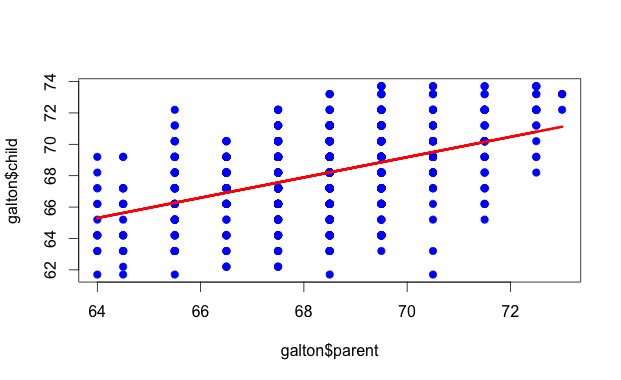
例としては、Rでお馴染みのgaltonのデータを使う。 これは、リンク先にも書いてあるけど、Galtonさんが1885に両親の身長と子供の身長の関係を分析したデータセットで、928サンプルが含まれている。RのUsingRパッケージに含まれているので、これをRで以下のようにして、galton.csvに保存しておく。
> install.packages("UsingR")
> library(UsingR)
> data(galton)
> write.csv(galton, "galton.csv", row.names = FALSE)
せっかくなので、Rで線形回帰をして散布図上にプロットしておく。
> lm <- lm(galton$child ~ galton$parent)
> summary(lm)

Call:
lm(formula = galton$child ~ galton$parent)

Residuals:
    Min      1Q  Median      3Q     Max
-7.8050 -1.3661  0.0487  1.6339  5.9264

Coefficients:
              Estimate Std. Error t value Pr(>|t|)
(Intercept)   23.94153    2.81088   8.517   <2e-16 ***
galton$parent  0.64629    0.04114  15.711   <2e-16 ***
---
Signif. codes:  0 ‘***’ 0.001 ‘**’ 0.01 ‘*’ 0.05 ‘.’ 0.1 ‘ ’ 1

Residual standard error: 2.239 on 926 degrees of freedom
Multiple R-squared: 0.2105,	Adjusted R-squared: 0.2096
F-statistic: 246.8 on 1 and 926 DF,  p-value: < 2.2e-16

> plot(galton$parent, galton$child, pch=19, col="blue")
> lines(galton$parent, lm$fitted, col="red", lwd=3)
自動微分のコード
Conal Elliott のコードを使おうかと思ったけれど、Hackageにekmettプロダクトのadパッケージがあったので、それを使うことに。バージョンは3.4を使う。 そういえば、先日開催されていたekmett勉強会でも、@nebutalabという方がadの紹介をしていた。
最急降下法
で、grad関数で自動微分して勾配を求めて、それを使って最急降下法するコードを自分で書こうと思ったら、ちょうど都合の良いことにgradientDescentという関数が用意されていた。 なので、これを使うことにして書いてみたのが以下のコード。 gradientDescentには普通に目的関数costと初期値を引き渡しているだけで、勾配を計算するための関数などを全く引き渡していないことに注目。
-- Galton.hs
module Main where

import Control.Monad
import Numeric.AD
import Text.Printf
import qualified Text.CSV as CSV

main :: IO ()
main = do
  Right csv <- CSV.parseCSVFromFile "galton.csv"
  let samples :: [(Double, Double)]
      samples = [(read parent, read child) | [child,parent] <- tail csv]
      -- hypothesis
      h [theta0,theta1] x = theta0 + theta1*x
      -- cost function
      cost theta = mse [(realToFrac x, realToFrac y) | (x,y) <- samples] (h theta)
  forM_ (zip [(0::Int)..] (gradientDescent cost [0,0])) $ \(n,theta) -> do
    printf "[%d] cost = %f, theta = %s\n" n (cost theta :: Double) (show theta)

-- mean squared error
mse :: Fractional y => [(x,y)] -> (x -> y) -> y
mse samples h = sum [(h x - y)^(2::Int) | (x,y) <- samples] / fromIntegral (length samples)
実行結果
それで、コンパイルして実行してみると……
[0] cost = 3156.057306315988, theta = [2.6597058526401096e-2,1.8176025390625015]
[1] cost = 2146.158122210389, theta = [4.6848451721258726e-3,0.3193588373256373]
[2] cost = 1459.9671459993929, theta = [2.2758658044906822e-2,1.5543558052476183]
[3] cost = 993.724511817967, theta = [7.872126807824226e-3,0.5363518751316139]
[4] cost = 676.9290401789791, theta = [2.0154694031410444e-2,1.3754888484523264]
[5] cost = 461.6776592383078, theta = [1.0041866689573948e-2,0.6837909525010937]
[6] cost = 315.42191649062323, theta = [1.8389486179011837e-2,1.2539549823963831]
[7] cost = 216.0462832295627, theta = [1.1520222735584755e-2,0.783970560056418]
[8] cost = 148.52403553080242, theta = [1.719418363575862e-2,1.1713769350191798]
[9] cost = 102.64504299700745, theta = [1.252880777988588e-2,0.8520390200495115]
…
[100] cost = 5.391540483678139, theta = [1.5252813280501425e-2,0.9963219150471427]
[101] cost = 5.391540272870362, theta = [1.5259169016306468e-2,0.9963197390947276]
[102] cost = 5.391540062688162, theta = [1.5265580330093717e-2,0.9963213622860531]
[103] cost = 5.3915398529310075, theta = [1.5271945828031475e-2,0.9963198538562846]
[104] cost = 5.391539446704301, theta = [1.5284752349382588e-2,0.996321999765866]
…
[1000] cost = 5.3913214546153885, theta = [2.195100305728909e-2,0.9962239448356897]
[1001] cost = 5.39132107512034, theta = [2.19637098242177e-2,0.9962195158083134]
[1002] cost = 5.391320924102971, theta = [2.1976643022454955e-2,0.996230564935548]
[1003] cost = 5.391320615754077, theta = [2.198280974693417e-2,0.9962155918323486]
[1004] cost = 5.391320339333709, theta = [2.1989373588151114e-2,0.9962277637190161]
…
[10000] cost = 5.389137897180453, theta = [8.88298535971496e-2,0.9952457730583962]
[10001] cost = 5.38913768668423, theta = [8.8836182876215e-2,0.9952431313378857]
[10002] cost = 5.389137477124735, theta = [8.884258017163454e-2,0.995245138984378]
[10003] cost = 5.389137268201876, theta = [8.884892139830691e-2,0.995243314173662]
[10004] cost = 5.389136870256361, theta = [8.886169628000305e-2,0.9952459827149522]
全然収束しない。収束遅すぎだろ。めげずにさらに放置してると……
[100000] cost = 5.367962167905593, theta = [0.7474196350908293,0.9856182795949244]
[100001] cost = 5.367961856713982, theta = [0.7474255920526732,0.9856022065240108]
[100002] cost = 5.367961582358961, theta = [0.7474319755635072,0.9856152902779793]
[100003] cost = 5.367961333033166, theta = [0.747438007468459,0.9856043401613668]
[100004] cost = 5.367961100713857, theta = [0.7474443291979176,0.9856132010817849]
…
[1000000] cost = 5.210315054542271, theta = [6.411550087218479,0.9027479380474824]
[1000001] cost = 5.210314936517216, theta = [6.411554713147153,0.9027442449249086]
[1000002] cost = 5.210314820386824, theta = [6.411559435811994,0.9027471642783936]
[1000003] cost = 5.210314705543812, theta = [6.411564078735267,0.9027446329906037]
[1000004] cost = 5.210314591575562, theta = [6.411568787386962,0.9027465946477329]
…
[5000000] cost = 5.0177281352658305, theta = [18.890815946868038,0.7201815311956332]
[5000001] cost = 5.017728123133143, theta = [18.890817258298373,0.7201790053001258]
[5000002] cost = 5.017728111906337, theta = [18.89081863661461,0.720181051408368]
[5000003] cost = 5.017728101294881, theta = [18.89081995979637,0.7201793288296293]
[5000004] cost = 5.01772809110162, theta = [18.890821328424636,0.7201807127666369]
…
[10000000] cost = 5.001070611475556, theta = [22.875383075131683,0.6618880826205324]
[10000001] cost = 5.00107061095209, theta = [22.87538335250446,0.6618875866914469]
[10000002] cost = 5.001070610463426, theta = [22.875383643001708,0.6618879878893927]
[10000003] cost = 5.001070609998513, theta = [22.875383922680363,0.6618876495886096]
[10000004] cost = 5.001070609549686, theta = [22.87538421127661,0.6618879208540909]
まだかかるのかよ……
[15000000] cost = 5.000328380487849, theta = [23.716478910924902,0.6495830291863548]
[15000001] cost = 5.0003283804652, theta = [23.71647896958202,0.6495829318117019]
[15000002] cost = 5.000328380443848, theta = [23.71647903081446,0.6495830104741416]
[15000003] cost = 5.000328380423461, theta = [23.716479089924043,0.6495829440298111]
[15000004] cost = 5.000328380403642, theta = [23.71647915078346,0.649582997196493]
…
[20000000] cost = 5.0002953079344685, theta = [23.894024471635685,0.6469855785633368]
[20000001] cost = 5.000295307933508, theta = [23.894024484038532,0.64698555944479]
[20000002] cost = 5.000295307932569, theta = [23.89402449694667,0.6469855748657359]
[20000003] cost = 5.0002953079316805, theta = [23.894024509438292,0.6469855618158963]
[20000004] cost = 5.000295307930787, theta = [23.89402452227324,0.6469855722344278]
…
[22987995] cost = 5.000294005873883, theta = [23.922778217862263,0.6465649143875803]
[22987996] cost = 5.000294005873744, theta = [23.922778220364872,0.6465649143543949]
[22987997] cost = 5.000294005873735, theta = [23.922778220366094,0.6465649143543771]
[22987998] cost = 5.000294005873733, theta = [23.922778220367316,0.6465649143543594]
[22987999] cost = 5.000294005873733, theta = [23.922778220367316,0.6465649143543594]
[22988000] cost = 5.000294005873733, theta = [23.922778220367316,0.6465649143543594]
やった! 収束した!
Rだと一瞬だったところ、1.5日くらいかかったし、Rで計算した theta0=23.94153, theta1=0.64629 とはちょっとずれてはいるけれど。
感想
Courseraの Machine Learning のコースで、最急降下法で線形回帰を実装したときは1000ステップくらいで収束してたので、これもそれくらいで収束するかと思ってたんだけれど、こんなにかかるとは以外だった。 gradientDescent関数(ソース)の実装に何か問題があるのか、それともそもそも素朴な最急降下法には荷の重い問題だったのか分からんけれど、2パラメータのこの程度の問題でこれは流石に酷い。
本当はこの後は、ロジスティック回帰とニューラルネットの例も何かやってみようかと思ってたのだけれど、その前にそっちを何とかしないといけないかも。 Machine Learning のコースでも最初は簡単な再急降下法を自前で実装させていたけれど、その後は最適化は予め用意してある実装(fmincg.m)を使うようになってたからなぁ。 まあ、時間かかりすぎて疲れたので、また今度。
【追記】頂いたコメンドなど
これは中で使ってる勾配法のステップ設定が狂っている感.このデータなら単純な勾配法でもここまで収束遅くはないと思われる.
— Takanori MAEHARA (@tmaehara) November 27, 2013目的関数値の減少量はステップ幅と同じくらいのオーダーのはずだから,ステップ幅のスケジューリングが急すぎるとかかしらん…….
— Takanori MAEHARA (@tmaehara) November 27, 2013【追記】 解決策
- conjugated gradient descent などのより賢い最適化手法を使う → nonlinear-optimizationパッケージで遊ぶ (ヒビルテ 2013-11-28)
- データのスケーリング → コメント欄参照
- 勾配法のステップ設定 → ?
2013-11-28 [長年日記]
λ. nonlinear-optimizationパッケージで遊ぶ
「自動微分を使って線形回帰をしてみる」の続きで、最急降下法を自分で書いてみるかと思ったのだけれど、そういえばHackageにnonlinear-optimizationパッケージというのがあったのを思い出した。以前から、一回試してみたいと思っていたパッケージだったので、せっかくなのでこれを試してみる。 試してみるバージョンは現時点での最新版の0.3.7で、Hager and Zhang *1 のアルゴリズムを同著者らが実装したCG_DESCENTライブラリのバインディングが提供されている。
nonlinear-optimizationパッケージのAPIはadパッケージのgradientDescent関数に比べるとちょっと面倒臭いAPIだけれど、前回のコードを書き換えてみたのが以下のコード。 nonlinear-optimizationパッケージは自動微分とかはしないので、勾配を計算する関数を明示的に渡す必要があり、adパッケージのgrad関数で自動微分した結果の関数を渡すようにしてある。
module Main where

import Control.Monad
import qualified Data.Vector as V
import Numeric.AD
import qualified Numeric.Optimization.Algorithms.HagerZhang05 as CG
import Text.Printf
import qualified Text.CSV as CSV

main :: IO ()
main = do
  Right csv <- CSV.parseCSVFromFile "galton.csv"
  let samples :: [(Double, Double)]
      samples = [(read parent, read child) | [child,parent] <- tail csv]
      -- hypothesis
      h theta x = (theta V.! 0) + (theta V.! 1) * x
      -- cost function
      cost theta = mse [(realToFrac x, realToFrac y) | (x,y) <- samples] (h theta)
  (theta, result, stat) <-
    CG.optimize
      CG.defaultParameters{ CG.printFinal = True, CG.printParams = True, CG.verbose = CG.Verbose }
      0.0000001                  -- grad_tol
      (V.fromList [0::Double,0]) -- Initial guess
      (CG.VFunction cost)        -- Function to be minimized.
      (CG.VGradient (grad cost)) -- Gradient of the function.
      Nothing                    -- (Optional) Combined function computing both the function and its gradient.
  print theta

-- mean squared error
mse :: Fractional y => [(x,y)] -> (x -> y) -> y
mse samples h = sum [(h x - y)^(2::Int) | (x,y) <- samples] / fromIntegral (length samples)
で、これを実行してみると……
PARAMETERS:

Wolfe line search parameter ..................... delta: 1.000000e-01
Wolfe line search parameter ..................... sigma: 9.000000e-01
decay factor for bracketing interval ............ gamma: 6.600000e-01
growth factor for bracket interval ................ rho: 5.000000e+00
growth factor for bracket interval after nan .. nan_rho: 1.300000e+00
truncation factor for cg beta ..................... eta: 1.000000e-02
perturbation parameter for function value ......... eps: 1.000000e-06
factor for computing average cost .............. Qdecay: 7.000000e-01
relative change in cost to stop quadstep ... QuadCufOff: 1.000000e-12
factor multiplying gradient in stop condition . StopFac: 0.000000e+00
cost change factor, approx Wolfe transition . AWolfeFac: 1.000000e-03
restart cg every restart_fac*n iterations . restart_fac: 1.000000e+00
stop when cost change <= feps*|f| ................. eps: 1.000000e-06
starting guess parameter in first iteration ...... psi0: 1.000000e-02
starting step in first iteration if nonzero ...... step: 0.000000e+00
factor multiply starting guess in quad step ...... psi1: 1.000000e-01
initial guess factor for general iteration ....... psi2: 2.000000e+00
max iterations is n*maxit_fac ............... maxit_fac: 1.797693e+308
max expansions in line search ................. nexpand: 50
max secant iterations in line search .......... nsecant: 50
print level (0 = none, 2 = maximum) ........ PrintLevel: 1
Logical parameters:
    Error estimate for function value is eps
    Use quadratic interpolation step
    Print final cost and statistics
    Print the parameter structure
    Wolfe line search ... switching to approximate Wolfe
    Stopping condition uses initial grad tolerance
    Do not check for decay of cost, debugger is off
iter:     0 f =   4.642373e+03 gnorm =   9.306125e+03 AWolfe =  0
QuadOK:  1 initial a:   1.070618e-04 f0:   4.642373e+03 dphi:  -8.662251e+07
Wolfe line search

iter:     1 f =   5.391563e+00 gnorm =   3.269753e-02 AWolfe =  0
QuadOK:  1 initial a:   1.632104e+01 f0:   5.391563e+00 dphi:  -1.069411e-03
Wolfe line search
RESTART CG

iter:     2 f =   5.387312e+00 gnorm =   1.558689e+01 AWolfe =  1
QuadOK:  0 initial a:   3.264209e+01 f0:   5.387312e+00 dphi:  -2.430188e+02
Approximate Wolfe line search

iter:     3 f =   5.374303e+00 gnorm =   3.196800e-02 AWolfe =  1
QuadOK:  1 initial a:   3.559386e+00 f0:   5.374303e+00 dphi:  -1.022238e-03
Approximate Wolfe line search
RESTART CG

iter:     4 f =   5.288871e+00 gnorm =   2.808049e-02 AWolfe =  1
QuadOK:  1 initial a:   2.376426e+01 f0:   5.288871e+00 dphi:  -7.887345e-04
Approximate Wolfe line search

iter:     5 f =   5.279499e+00 gnorm =   1.301306e+01 AWolfe =  1
QuadOK:  0 initial a:   4.752853e+01 f0:   5.279499e+00 dphi:  -1.693871e+02
Approximate Wolfe line search
RESTART CG

Termination status: 0
Convergence tolerance for gradient satisfied
maximum norm for gradient:  5.513258e-09
function value:             5.000294e+00

cg  iterations:                   6
function evaluations:            15
gradient evaluations:            11
===================================

fromList [23.941530180694265,0.6462905819889333]
今度は一瞬で収束した! やった!
*1 Hager, W. W. and Zhang, H. A new conjugate gradient method with guaranteed descent and an efficient line search. Society of Industrial and Applied Mathematics Journal on Optimization, 16 (2005), 170-192.

ψ mkotha [入力をおおざっぱに正規化(68を引いてから4で割る)してから最適化したところ、99ステップで(Doubleの最後の桁..]
ψ sakai [おお〜! そういえば、Courseraの講義でも feature scaling が勾配法の収束の速度に効いてくると..]